Introduction – Flexibility of Shell Models
Shell models are probably the most-used FE (Finite Element) engineering model in civil engineering and mechanical engineering. Shells are like volumetric FEs with a single layer. In the thickness direction, they behave like beams. They have the same advantages and disadvantages as beams. Shells do not give the right solution near supports, plate intersections, or concentrated loads like point loads and line loads.
FEM-Design, however, has slightly different shell models which partly overcome this limitation that other software usually has. A huge benefit of shell models is that they are ultimately more accurate in describing bending than volumetric FE models. When there is no FE discretisation in the plate depth direction, division does not affect the bending response. Usually, when volumetric FEs are used in a plate-like element, there are only two nodes in the depth direction, and even higher-order elements are somewhat inaccurate. First-order volumetric elements cannot describe plate bending. So shell models are a perfect solution for plate-like structures such as concrete walls, plates, glass fiber composites, timber plates, steel-plated welded structures, and similar systems. If you have only used volumetric FEs, you do not know what you are missing: shells are incredible for describing engineering systems. You can directly manipulate in-plane shear stiffness, torsional stiffness, or compression-bending x-y interaction. These manipulations, which are needed in practical engineering systems, are close to impossible with volumetric FEs.
One huge advantage of shells is that they are cross-sectional models, like beams. You get forces acting directly over the system section. Result take-out is easy. Applying advanced section-capacity design formulas is much easier than with solid FEs, where depth-direction integration is needed to get system bending, shear, or any other design value.
Shells are like beam FEs for describing bending, but there is a huge caveat: the common misconception is that shells are like 2 beam grids perpendicular to each other. This is not the correct mental model for shells and has caused a lot of confusion. This article explains the correct way to think about shells. Once you understand how shells work, you can set their properties and build your own formulas and engineering models. Many have used shell FEs for years without any deeper thinking about their inner workings – but it pays to understand them.
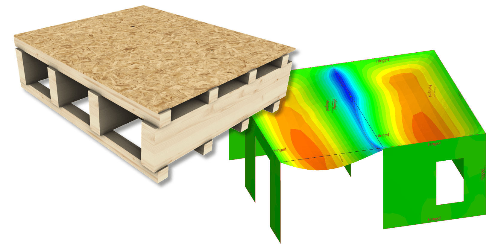
Example 1: System with high bending x stiffness, low bending y stiffness, low torsional stiffness, moderate to low interaction between x and y bending – difficult to model with volumetric FEs taking into account connector slip but can be done very easily by composing an equivalent shell model: right.
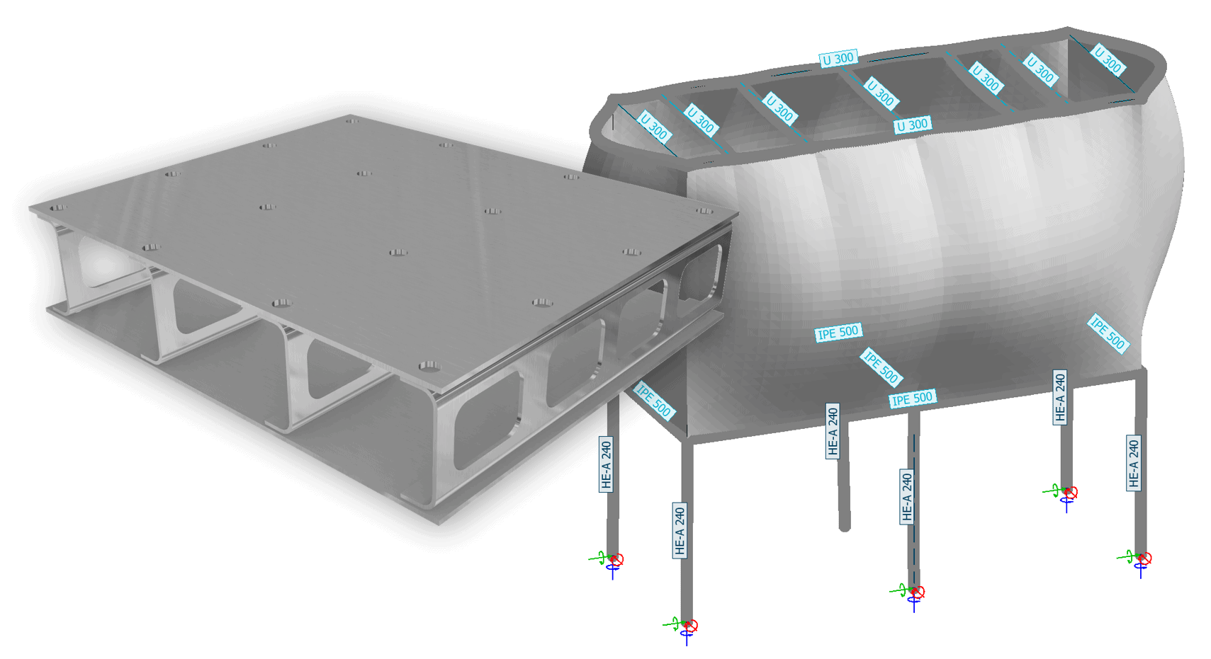
Example 2: Left: complex structure system. Right – Equivalent shell model simplification of a system with high bending x, moderate torsion stiffness, low shear stiffness y.
Twist of shells – So Much Confusion
First, we’ll talk about shell twist stiffness, even though it might be the property causing the most confusion. Twist stiffness can usually be handled alone without coupling (explained later). A common misconception about shell models is that shell bending behaviour can be explained by two bending stiffnesses, bending x and bending y. While this model is valid for certain cases, it cannot explain most real-world plate-like systems. The best real-world analogy I could think of for this “bending alone” model is a stack of pipes with 2 perpendicular layers. While this stack has bending stiffness in the x and y directions, one stiffness is zero. And that is twist – moving one corner from a flat plane. It does not require any bending deformation of pipes. Twist stiffness is needed to provide this stiffness against this deformation mode – at least for those systems where this stiffness is high.
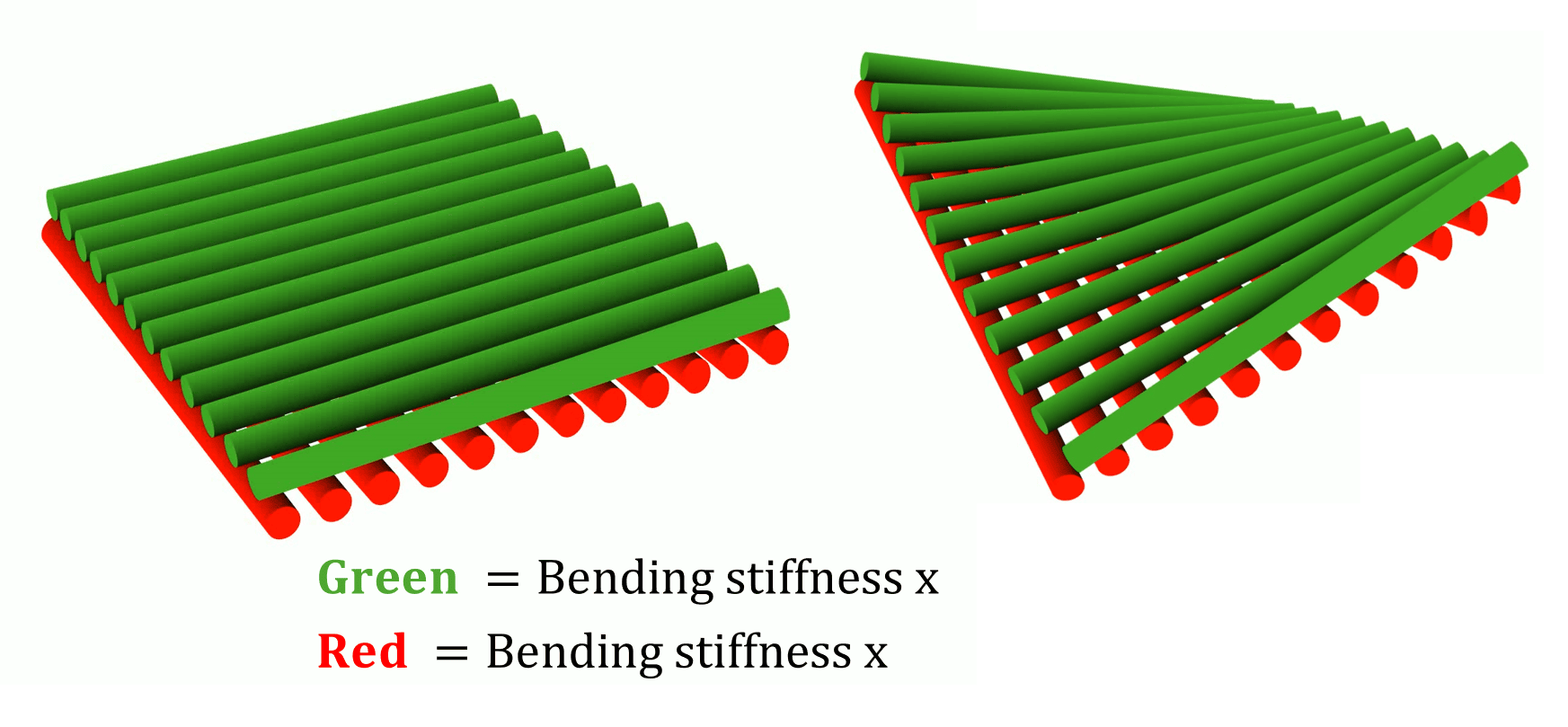
Concept: Bending stiffness in 2 directions alone makes the system unstable with twist loading. These systems exist as ideal models. 2-layer stack of pipes vertically connected as an analogy.
Twist moment, usually Mxy in FE results, is also a source of confusion. I have heard many times that shell twist is just bending that happens at a 45-degree angle to the shell’s main axes. Another popular explanation of shell twist is saddle-type deformation of shells. As simple and elegant as these explanations are, both are incorrect or at least only part of the equation. First, let’s look at the principal bending moments M1 and M2 (directions of max and min bending, which are 90 deg. apart in the shell-twist case). Image below. In the twist case, the principal bending moments are roughly at a 45-degree angle to the main axes, so there is some truth to the first simple explanation. Also, look at the definition of twist moment.
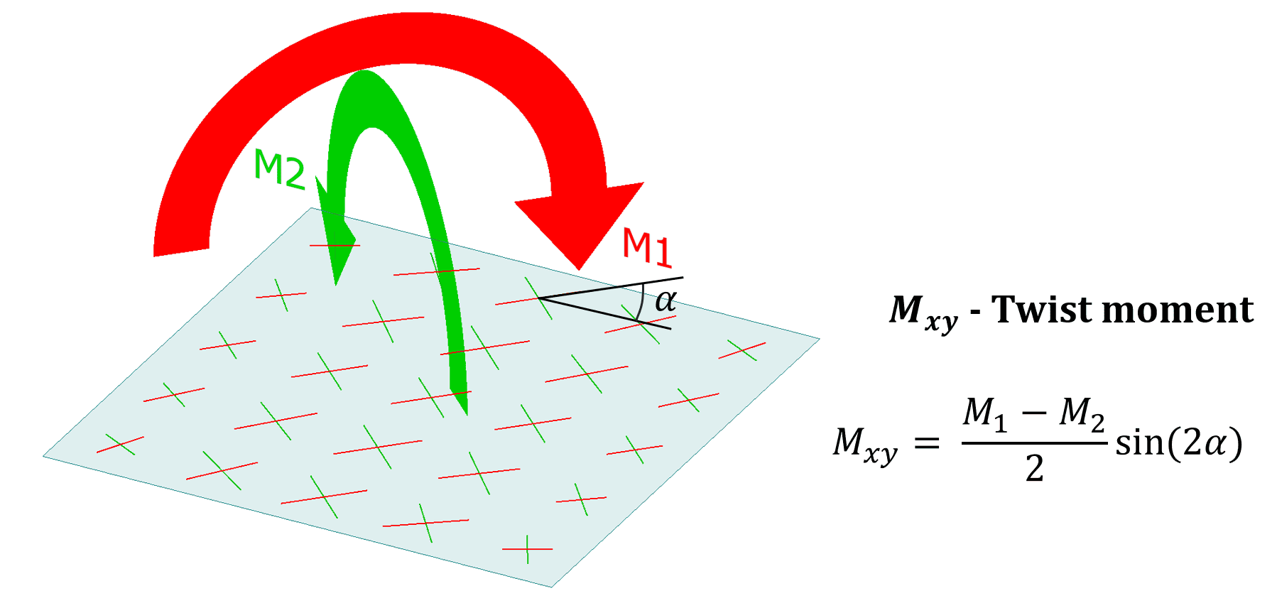
Image of principal bending moments of a shell model under twist load and definition of twist moments Mxy.
You can get an even better understanding by defining a shell with very low twist stiffness and studying its response under different loads. The image below illustrates this. If we apply saddle deformation (bottom left), we can see that saddle deformation is not the answer to shell twist. If we apply 45-degree angle bending to the shell (top right), we see that the system still has stiffness. Also, this stack of pipes has stiffness in both cases. When both are bending at a 45-degree angle and a saddle shape happens, the system loses stiffness. So, shell twist stiffness “KGxy” is the system’s stiffness against a difference in principal bending moment when bending is not parallel to the shell axes. Also, the Mxy formula below explains that. Mxy (twisting moment) happens only if there is a difference in M1 and M2, and the twisting moment max is when bending is in a 45-degree direction. So, in layman’s terms, we can say twisting stiffness is the glue that keeps this pipe stack from twisting. If you understand all this, you probably understand shell twisting better than the average engineer.
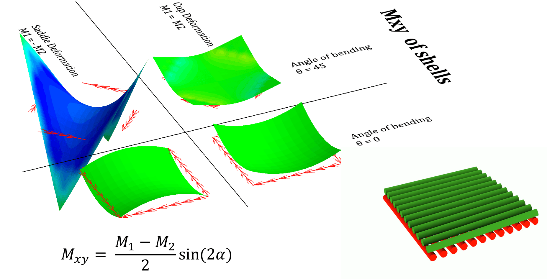
Image: what happens if different loading is applied to a shell with reduced twist stiffness. Colormap= shell Mx moment. Only one loading case shows Mxy internal force and Mxy deformation. Twisting moment Mxy happens only when bending has an angle to the main axes and principal moments are not equal. Pure twist is M1 = -M2.
Twist Deformation
It is obvious how bending deformation and compression deformation are calculated, and probably everyone has done so much beam bending math plus beam bending moment tables that I do not go into the calculation of those here. For shell twist, however, you must define the relationships between stiffness KGxy, internal force Mxy, and deformation – just like bending. This relationship defines twist curvature. For actual deformation in the shell thickness direction, which is easier to obtain from an FE model, it has to be taken into account that twist deformation happens as a change in both the x and y directions of the shell. This relationship between KGxy, Mxy, and out-of-plane deformation z is useful when the deformation of a system under twist load (Mxy, calculated from principal moments) is known from a real test or a detailed 3D model.
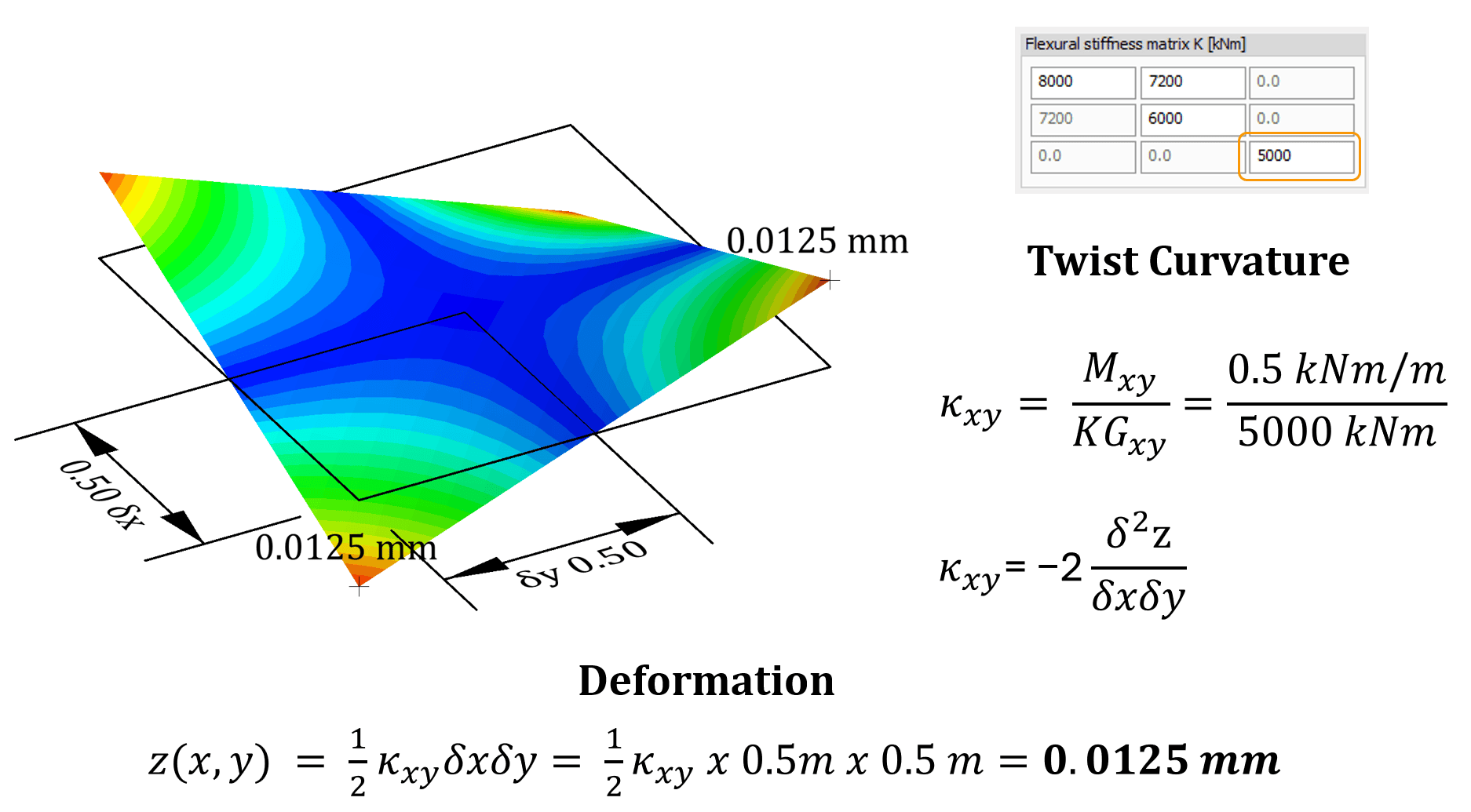
Image: Calculation of shell thickness direction out-of-plane deformation with shell KGxy and Twist moment Mxy.
Where Does Shell Twist Stiffness Come From
When a 3D body is twisted, principal bending moments occur at 45 degrees. The image below shows that both surfaces have a compression-tension biaxial stress state. This is pure shear stress (opposite N1 and N2). So twisting stiffness comes from the shear stiffness of plate layers. The mid-layer is stress-free, as in bending. For a continuum (no clear layers), stiffness comes from a constant change of shear stress through the thickness. This is not a universal definition and applies only when there is shear coupling between layers. Often real engineering systems do not have that shear coupling or have partial coupling. Without coupling, like a stack of papers, twisting stiffness is close to zero. Also, it is very obvious that coupled systems’ shear stiffness is directly proportional to how far apart, in the thickness direction, the shear-coupled plane-shear layers are.
Shell models, however, have “zero” thickness, so no real shear occurs in the shell’s top and bottom layers. All this shear-stress development in the layers is baked into the KGxy number, and shell stresses can be calculated in FE post-processing using the Mxy value and the distance from the centre of the shell. Please note that this post-processing usually works only for continuum models (solid plates). For other cases, you can calculate the skin shear from the Mxy force and add it to the bending and normal stresses.
Shell twist stiffness depends on:
- Shear stiffness of layers;
- Distance between layers;
- shear coupling in thickness direction between layers or skins.
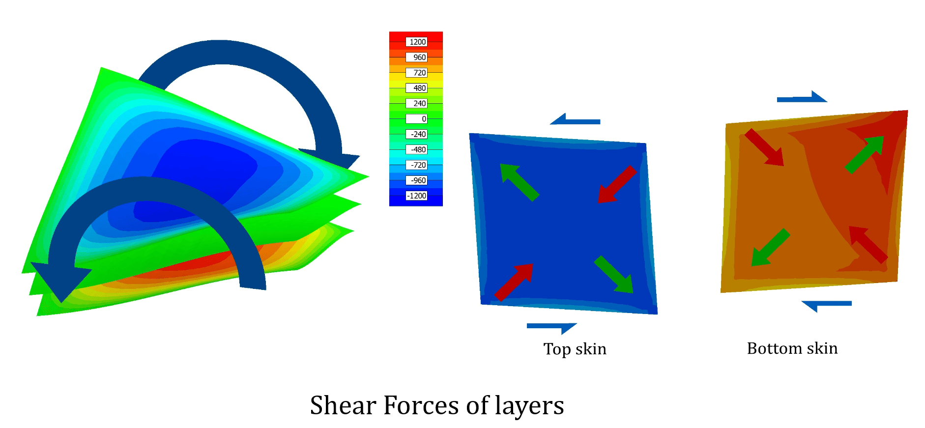
Image: Shear stresses of layers of a system under twist load. Top skin and bottom skin develop compression-tension at a 45-degree direction. This is a shear stress state (opposite principal stresses).
How to Calculate Twist Stiffness
The best starting point for calculating shell twist stiffness is to set aside standard formulas and think about how your engineering system works. Standard formulas work only for a solid plate. The best way to approach this is to use examples. The first case below is a solid plate like an uncracked concrete plate. The same formulas apply, of course, to steel plates (isotropic). The formulas below work for systems of non-shear-coupled layers. Single-layer twist stiffness, or so-called “self stiffness”, is the only component of twist stiffness. It’s only proportional to plane stress shear modulus G and thickness. All layers are summed up since there is no shear coupling. They have vertical coupling, so they naturally get the same shell twist curvature.
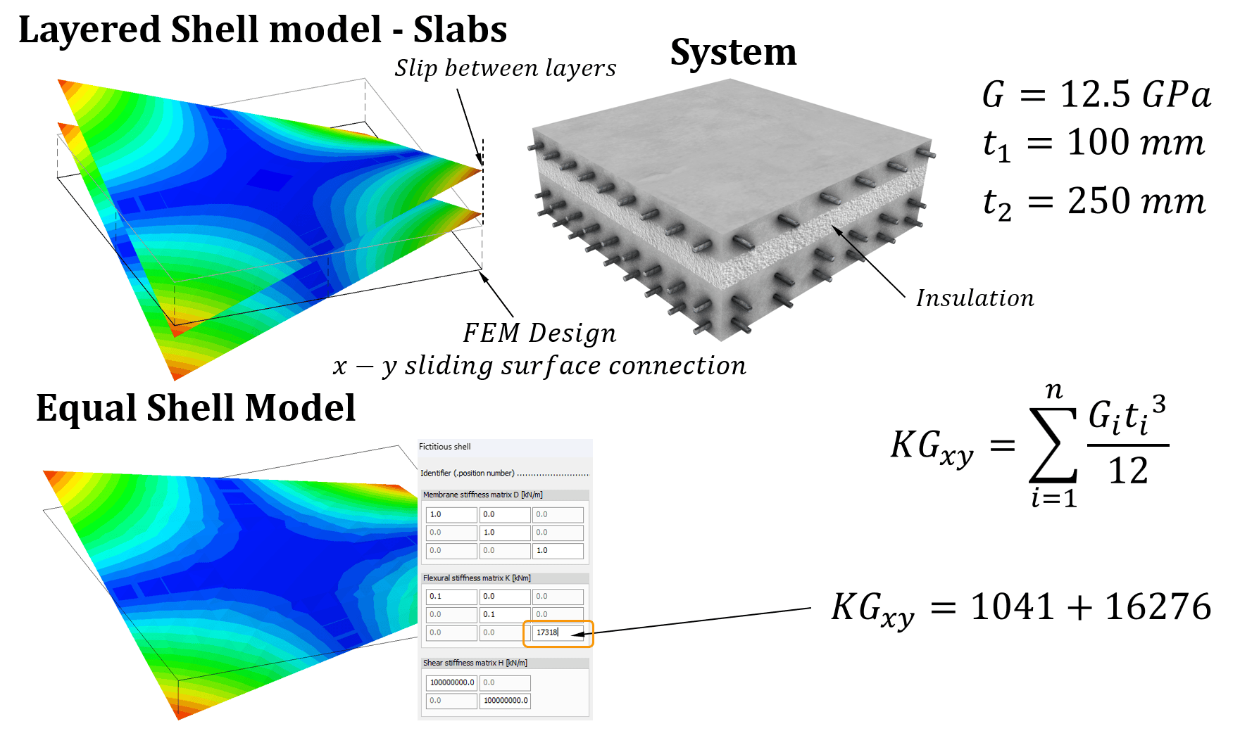
Image: Example calculation of solid shell twist stiffness. For shear un-coupled layers twist stiffness KGxy becomes just the sum of layers. Image also illustrates how FEM-Design can simulate the same system by defining two concrete plates (shells) and connecting them with a surface connection with zero x and y surface connection (sliding). Slip happens between layers, so twist stiffness is just the sum.
My personal favourite formula, which has served me well for 20 years, is the formula shown in the image below. This describes a system composed of two fully shear-coupled layers. This model is so handy since almost anything can be described by a system of two skins. And real engineering systems really are that. For example, a timber stud frame. Or a concrete slab. In the concrete example, one skin is surface rebar mesh, and the other is compressed concrete. The formula I have written below is simplified. It is very accurate for a system of plated thin skins. Twist stiffness of two-skin systems comes from two components: self-stiffness of the plate itself and composite effect caused by the distance between skins. The first component is usually minimal in these systems with strong shear coupling, so I have removed that part from the formula. This formula also works for systems like glass fiber composites with a foam core. Please note that this formula assumes full shear transfer.
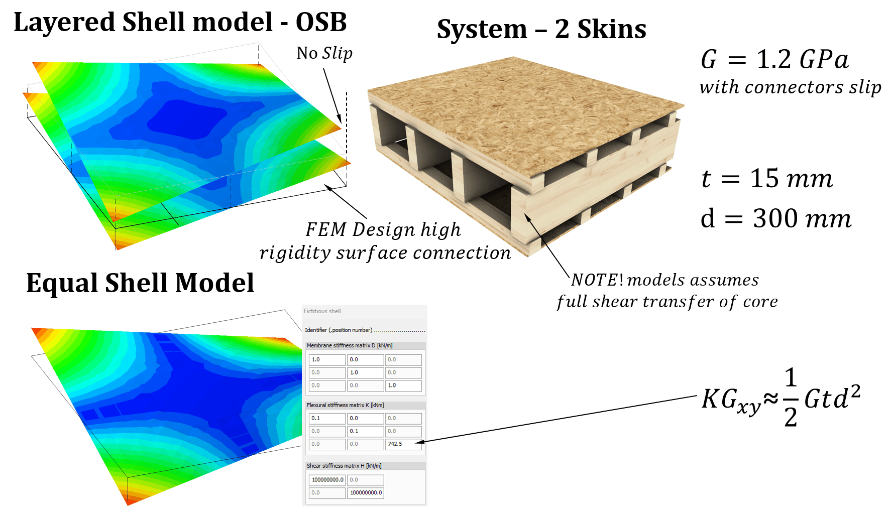
Image: Example calculation of two-skin twist stiffness with a simplified formula. FEM-Design can simulate the same system by defining two timber plates (shells) and connecting them with a surface connection with high x and y stiffness surface connection. As the image shows, shear slip is prevented. Two shells with surface connections match well with a simplified equal single shell with hand-calculated twist stiffness value.
Shell Twist Stiffness – Does it Matter?
The first reaction to complex structure mechanics topics is almost always to try to live without it. Unfortunately, twist stiffness is a real part of structural mechanics, and all plate-like structures have twist stiffness to some degree. When you understand what twist really is, it is easier to apply to daily design work. For example, the Wood & Armer equation is used for plate rebar design in bending. When you understand that twist causes tension at the surface, like bending, the coupling becomes clear, and so does the need to account for it in design. The image below illustrates this. However, FEM-Design uses all internal forces to calculate required rebar – not just My and Mxy, like the equation below. It is also worth noting that, especially in SLS checks, you can use twist response, and you need a correct model. The example image below is the vibration response of different types of timber floors.
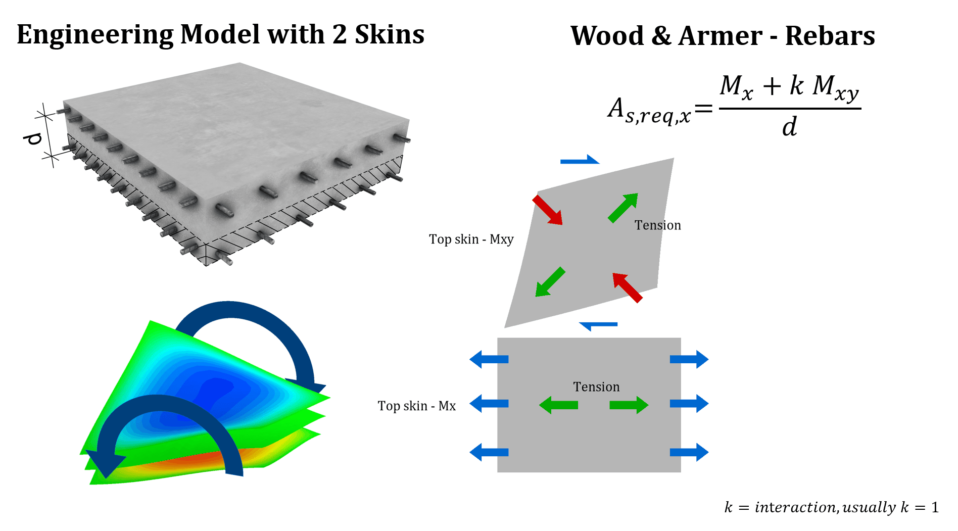
Image: Wood and Armer for plate rebar design. Effect of twist on required rebar. Both internal forces are needed for RC Design.
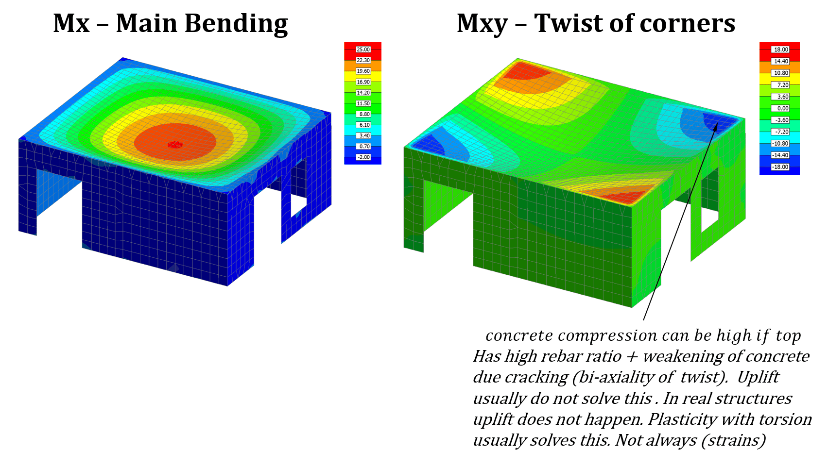
Image: RC plate and twist. Sometimes in design of these systems twist can be neglected. However, there is no universal rule when twist can be neglected. In some systems twist is the main load-bearing mechanism. Take bi-axiality of stresses caused by twist into account in plate design when checking concrete compression.
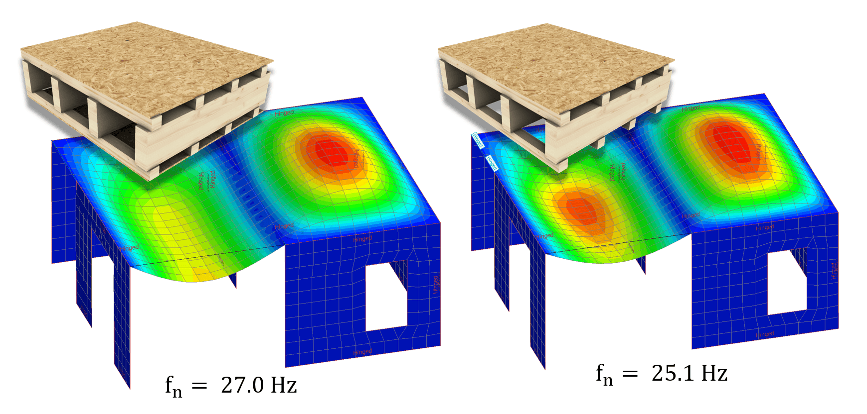
Image: Vibration of timber floor. Effect of twist stiffness of shells on frequency. The one on the left is an example of a two-skin system with high twist stiffness. To the right: system has only a single skin so only the self-stiffness component is left and that twist stiffness is close to zero – the plate works like an x-y beam grillage. Both models use beam stiffnesses as bending stiffness.
Plane Shear Stiffness of Shells
Shear stiffness can be the most important component of shell stiffness, or the least important. This all depends on the engineering system you are describing. For short buildings (1-3 stories), wall shear stiffness plays an important role in internal force distribution. For narrow and tall buildings, and for shaft and core wall systems, it is less significant. Of course, shear stiffness cannot be zero. Almost nothing is stable when shear stiffness is zero. In some systems, like stud frame walls with sheeting and timber floors with sheeting, shear stiffness almost always is the main contributor to deformation – there it is crucial what you define. For long beams made with shell elements without torsion and with thick and short section parts, shell shear stiffness has to be high – it’s not the main contributor to deformations. Shell Tension-compression terms matter only when the shell-model beam is short; when plated parts of the beam are wide and thin, in-plane shear stiffness contributes meaningfully to stiffness (shear deformation of the beam and shear lag of beams).
Shear Stiffness is closely related to twisting of shells – twisting is opposite shearing of opposite skins. Plane shear is same-direction shear of both skins. The image below illustrates why shear stiffness cannot be zero. The images also explain the relationship between FE-node deformation, Shear stiffness DGxy, and shell shear force.
You can understand the definition of shear force Nxy using the same pipe-stack analogy used above for shell twist. Shear Nxy is not the same as two different sign principal stresses. Shear is not compression at a 45-degree angle. This pipe stack below has stiffness when compressed or pulled vertically. It also has stiffness if all corners are pulled at a 45-degree direction outside from the centre. Shell shear stiffness is the stiffness to a difference in principal normal force when the direction is 45 degrees to the main fibers. Also, the definition of shear force Nxy is similar to Mxy.
Calculation of shear stiffness DGxy can be very simple for isotropic solid bodies. It is simply G x thickness. For single-skin or multiple-skin engineering systems, it is about the G modulus of plates and the slip modulus of connectors. For a very complex connector layout, like plug welds or plate connectors for drywall or OSB, the process is a bit more complex.
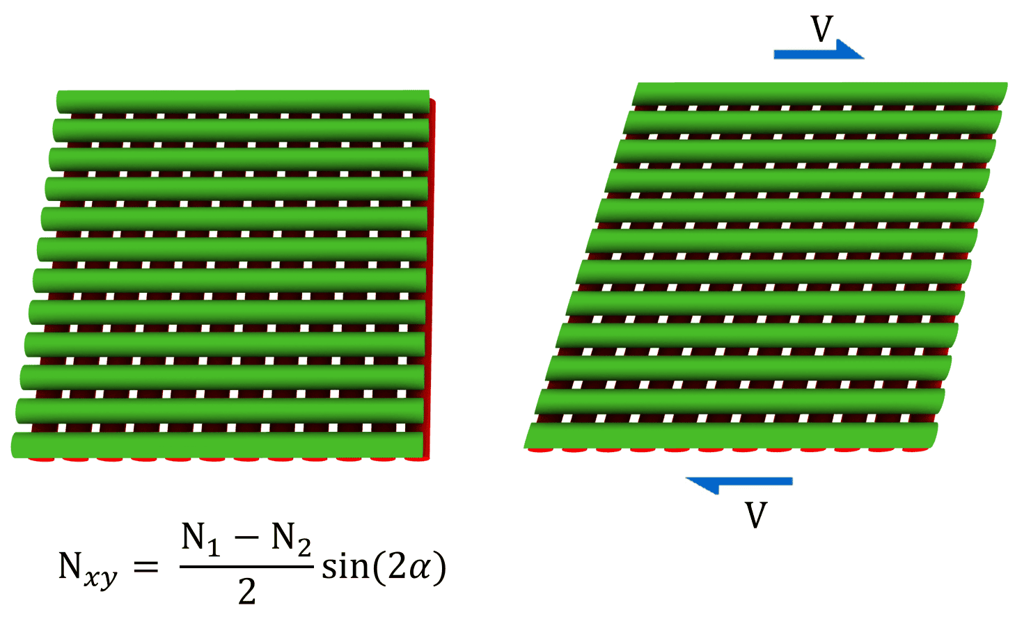
Image: Idealistic model of shear. Shear is the difference between N1 and N2 when N1 has an angle to main axes of shells. This pipe stack has stiffness with a difference in N1 and N2 only if it’s parallel to any main axes. In other cases, in-plane shear stiffness DGxy is needed.
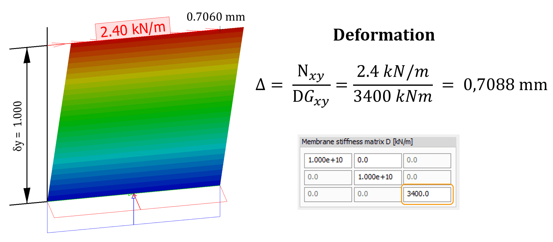
Image: Idealistic shell D matrix. High compression stiffness and limited shear stiffness. Link between DGxy value and deformation and shear force Nxy of shells. This link is needed if deformation is known from test data or a detail model.
Membrane Matrix and Coupling Factors
The membrane matrix of a shell describes its in-plane stiffness: two compression stiffnesses and one shear stiffness. Explanations of shell compression or tension stiffness fall short if they are not explained alongside coupling. Twisting stiffness and shear stiffness are the only stiffness components usually modelled in shells as individual components. A common misconception about shell compression stiffness is that it is just E x thickness. This gives too low a stiffness for the shell. The problem lies in the E value, which is measured from a real 3D body – it’s not a uniaxial spring, as many like to think. Poisson ratio causes coupling between compression x and y. This behaviour is modelled by coupling factors in the D matrix. So real 2D objects can be described by systems of coupled uni-axial springs. The image below illustrates the conversion factor from multi-axial E to the uniaxial spring system. So, instead of inputting E x t directly, remember to divide it by this correction factor.
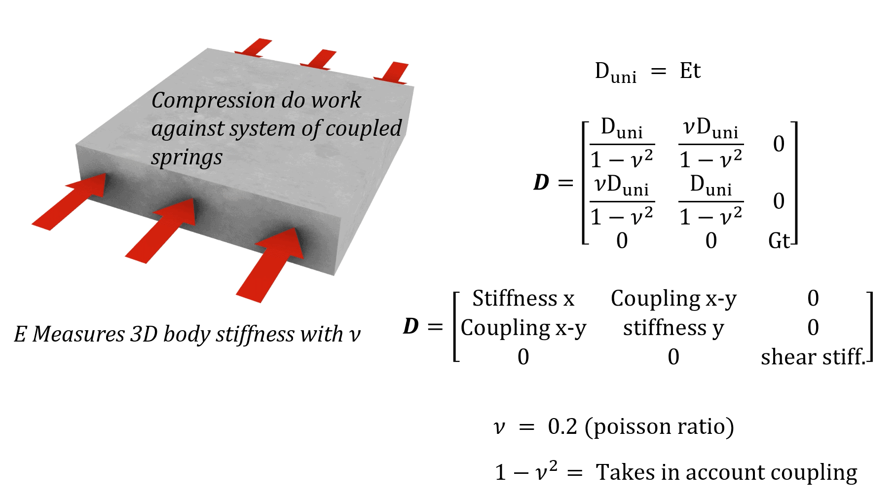
Image: Definition of isotropic D matrix with E and v and matrix components.
For Orthotropic complex systems (different compression stiffness in x and y directions), composed of a D matrix, it becomes a bit more interesting. The coupling factor in the matrix can no longer be calculated with the Poisson ratio. Instead, a new factor, “Rho,” is needed to replace the Poisson ratio. This new factor can be defined experimentally or using a detailed 3D model. The coupling term describes which kind of stiffness connection exists between x-spring values and y-spring values. Therefore, the coupling term is a function of both stiffnesses and this new factor “rho”. The D matrix is then constructed using the formulas in the image below.
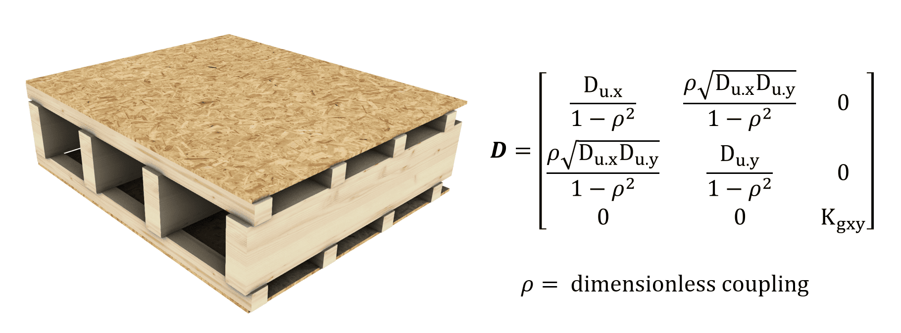
Image: Definition of orthotropic D matrix with x and y- compression stiffness (uniaxial stiffness) and coupling factor
Minimal Coupling with Compression?
Some real structure systems show little to no interaction. Also, when secondary stiffness is very low, coupling effects on the total system global response are minimal. Remember: coupling is a factor of the product of both stiffnesses, as per the equation above. A perfect FE shell model does not exist, but a reasonable engineering model can be done with what is known. A stud frame is a good example of this. Vertical compression causes minimal horizontal expansion of sheathing (OSB or drywall). When coupling is set to zero, you can input uniaxial stiffness (E x A) directly into the stiffness matrix. When rho is zero, the matrix really simplifies. Maybe the engineer wants the sheathing to take all lateral load, so it’s advisable to set twist stiffness to zero. Do you remember that shells have twist stiffness? Some lateral load is used to do work against shell twist, and if you don’t account for it in the design, it can be a problem.
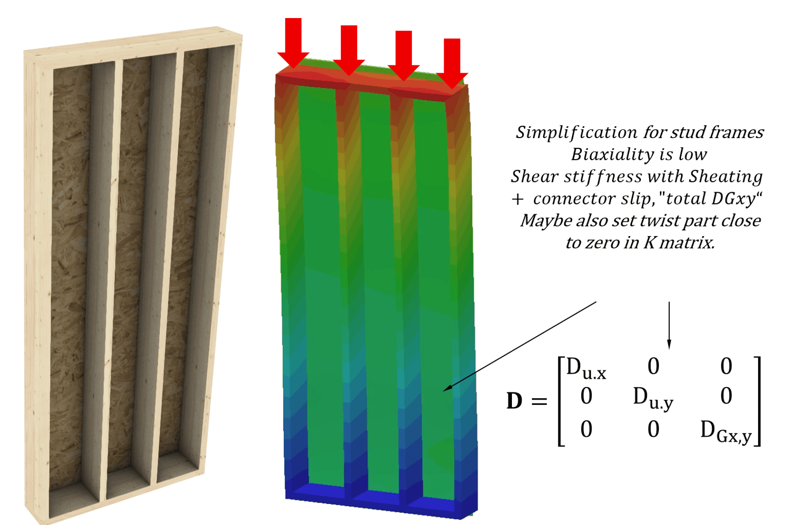
Image: idealised D matrix without coupling. Without coupling, E x A can be input directly into the matrix. FEM-Design allows very low stiffness values so that idealised models can be used.
Bending Matrix and Coupling
All that is said about the D matrix above is true for the bending matrix. Coupling also exists in bending. The image below illustrates this for a solid isotropic material. In this bending example, the top surface is under compression and the bottom under tension. Poisson ratio of the material causes perpendicular contraction in the bottom surface and expansion in the top. This means uniaxial bending does not exist in reality, not in beams and definitely not in slabs. For beams: the error is so small it can be neglected. Shell models must describe all this somehow; they do not have “bottom stresses” or “top stresses”. This is done with coupling terms in the K matrix (bending matrix). Also, uniaxial stiffness (beam bending stiffness) cannot be directly input into the K matrix because the K matrix describes a system of coupled uniaxial springs.
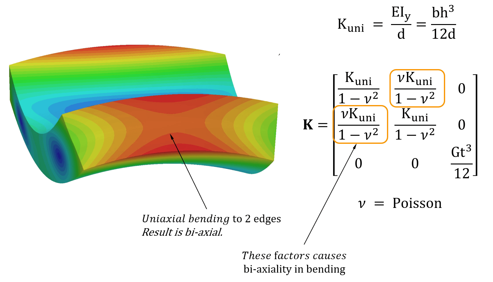
Image: Uniaxial bending to a real 3D object causes always bi-axial response. Matrix K with coupling factors is a way to describe this with shell FE. This image shows matrix and response of an isotropic solid.
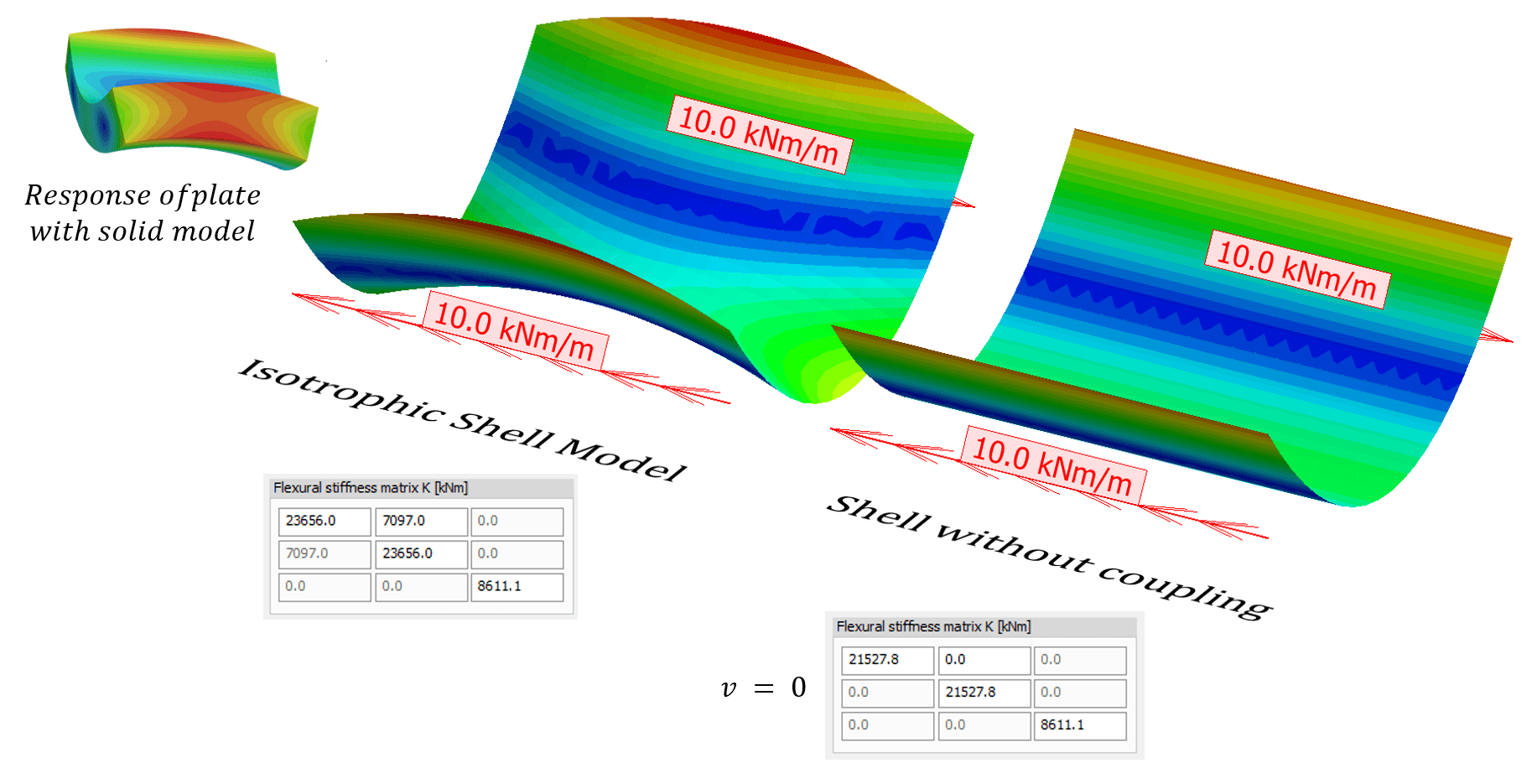
Image: How to replicate real system response with a shell model K matrix (left) and how to build an idealised engineering model (Right). Note also change in x and y-stiffnesses when coupling is removed.
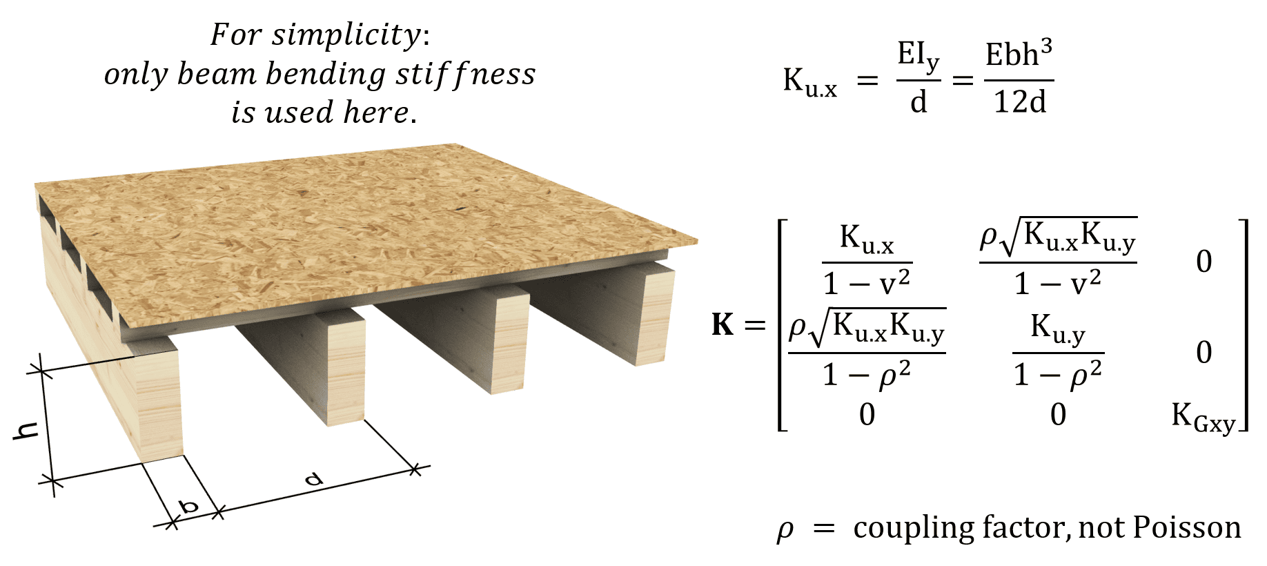
Image: General definition of orthotropic shell K matrix. The only unknown here is the rho factor which can be defined with a detailed model.
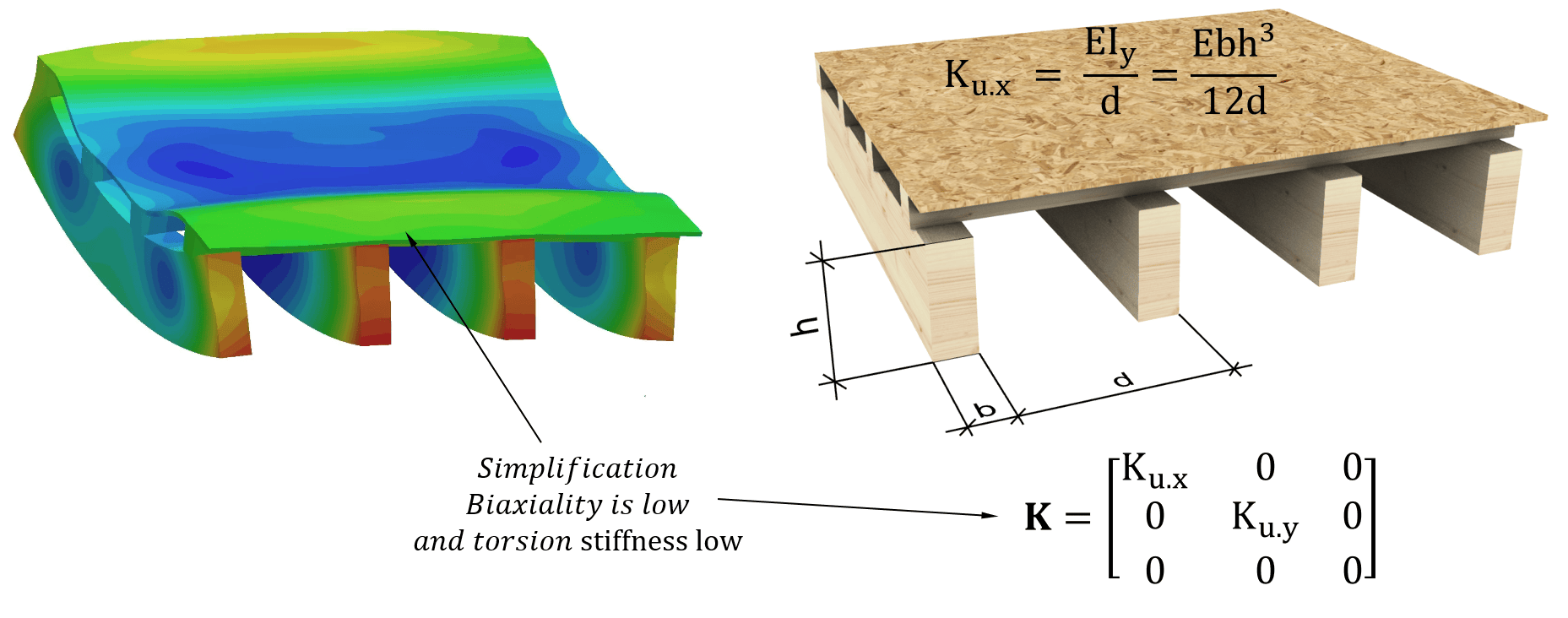
Image: response of the real system, detail. Idealised engineering model of floor with shells. When coupling is low the K matrix becomes simple. FEM-Design allows very low stiffness values: idealised models can be used.
Maximum and Minimum Coupling?
As you might know, the Poisson ratio has limits. At least for materials that we engineers really use. Zero Poisson ratio means a non-coupled material or a total ability to change volume under compression. This is close to open-cell materials and similar and like Styrofoam. A Poisson ratio larger than 0.5… if you do your math… means volume expansion under compression, which makes no sense. The normal range is 0.1–0.35. Also, the coupling term has limits. FEM-Design also checks coupling when you create a new shell, so it cannot create non-working FEs. Especially in cases with very different bending stiffnesses, the main bending is coupled with weaker bending, which makes no sense at all. This also applies to the D matrix. Realistic coupling term values are between 0.1 (Kx Ky)^0,5 and 0.4 (Kx Ky)^0,5. For ideal systems coupling is zero.
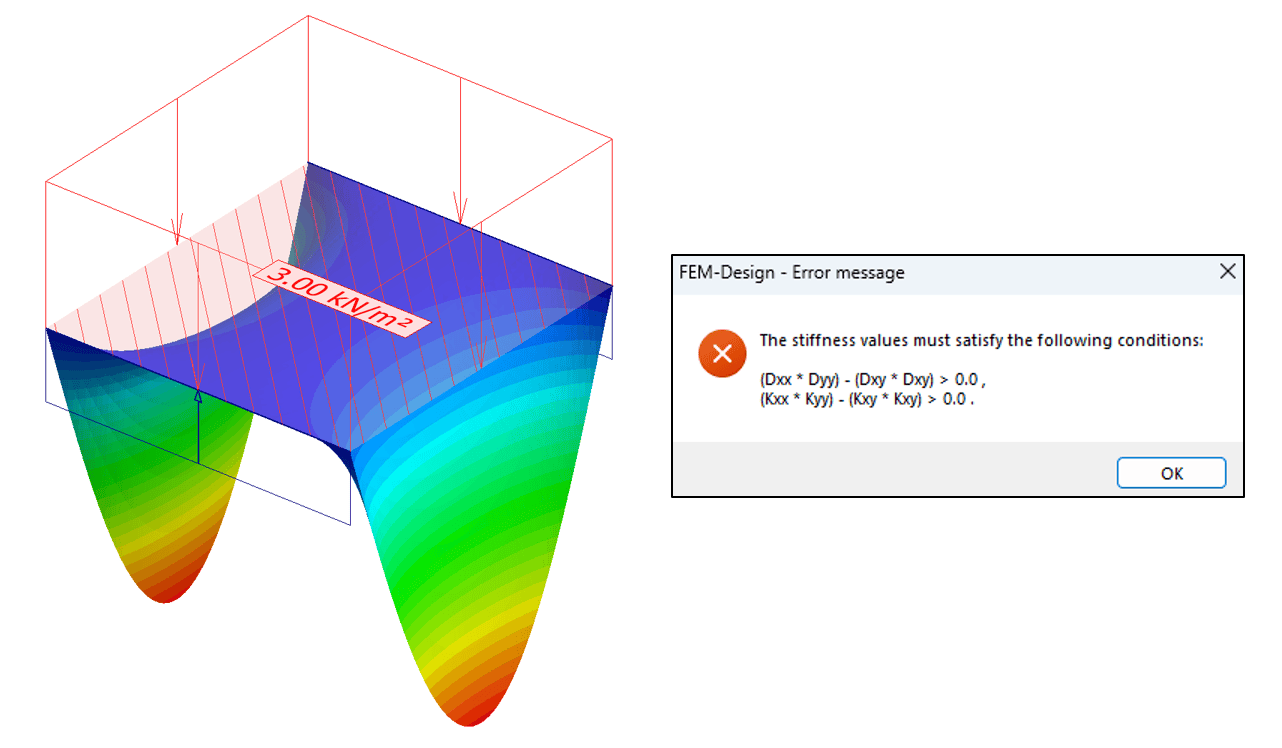
Image: Example of too high coupling term in the K matrix. Perpendicular stiffness is low to main bending stiffness. Symptom: curling up of edges. Right: FEM-Design checks also your coupling terms in K and D matrices. This is just a secondary backup. Real usable range of realistic coupling is much narrower and is mentioned above.
More Coupling Factors?
As more math-literate readers have noticed by now, K and D matrices are mostly empty. In special cases, those matrices are diagonal matrices, so there are only numbers in the diagonal from top left to bottom right of the matrix. This means there is no interaction between springs in the system. Usually, only bending coupling and compression couplings are essential to get the right response of real systems. But any coupling can be made with matrices. Only if it makes sense physically in a real structure: for example, twist will cause bending in x or similar coupling. One example of additional couplings used in FEM-Design is the coupling between shell compression and bending in CLT FE models. Coupling works both ways: pure compression causes curvature, and pure bending causes shortening of the element.
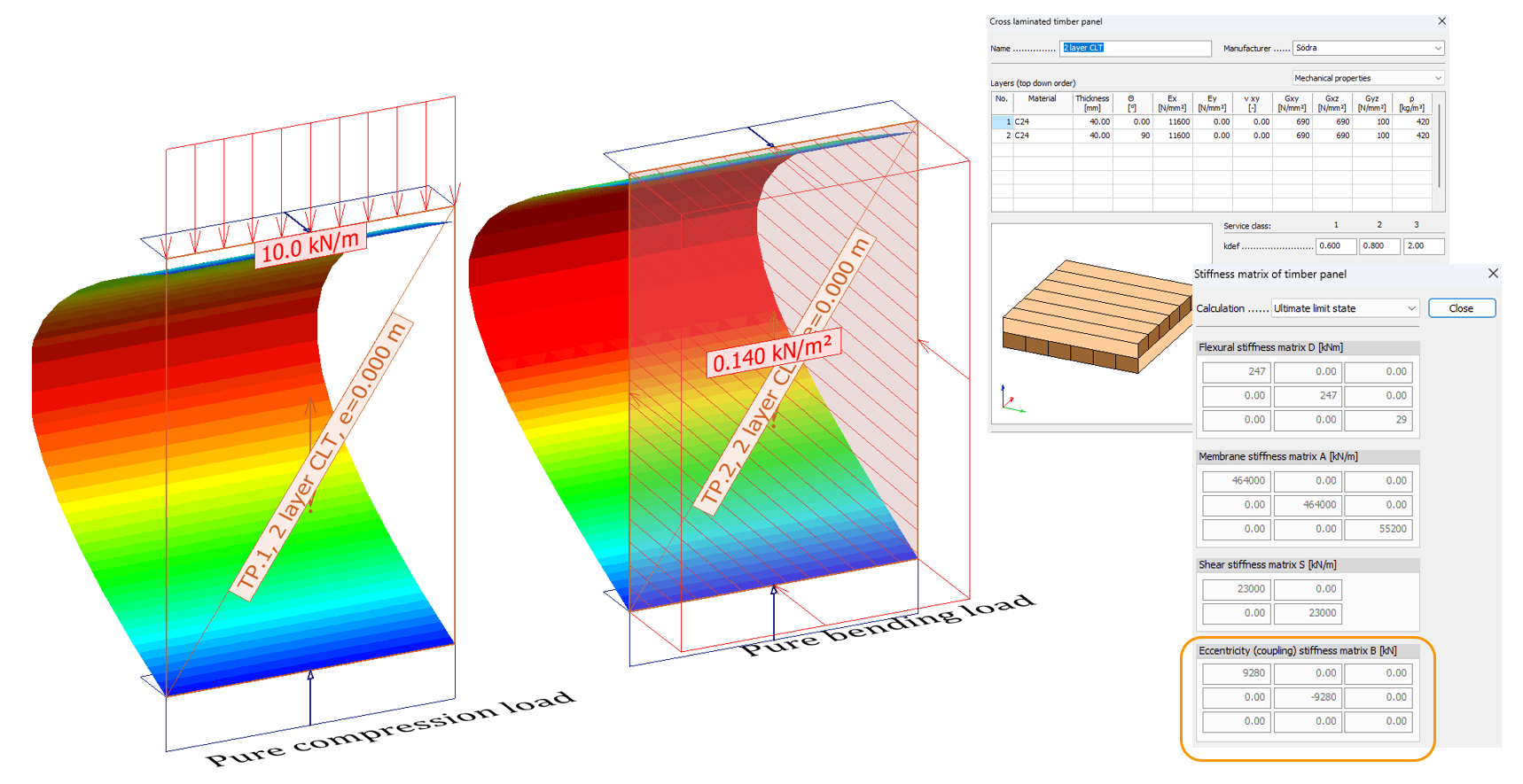
Image: Asymmetrical CLT panel in FEM-Design. Additional coupling factors between bending X and compression X springs. Coupling works both ways: compression causes curvature and bending causes shortening of the element. Note the different name of matrices in timber panels. The flexure matrix is called matrix D, not to be confused with membrane matrix D explained in this article (fictitious shell tool.
Do I Really Understand This?
The definition of a shell becomes very complex when more couplings are introduced. And the risk of errors and the risk of not understanding the system increase. Bending-normal-force coupling often causes unwanted diaphragm forces. Floor bends down, but in-plane shear carries load – not beams. It is often safer to assume fewer stiffness components. If twist stiffness is uncertain – reduce it or put it to zero. This is possible if ductility and the SLS criterion can be justified to distribute load to other stiffness components of the system. In the case of main torsion loading, this simplification, that torsion stiffness is zero, is not justified. But in the case of a timber floor supported on 4 sides where torsion stiffness is uncertain, probably some plasticity of connectors can allow large torsional deformation to change the system to a pure biaxial system. So, you can simplify the system by eliminating torsion stiffness. The point of building these systems is to do engineering where safety and transparency are main principles. Simplify when possible without adding risk. And it all comes back to the original theme of this blog – understand systems instead of using equations.
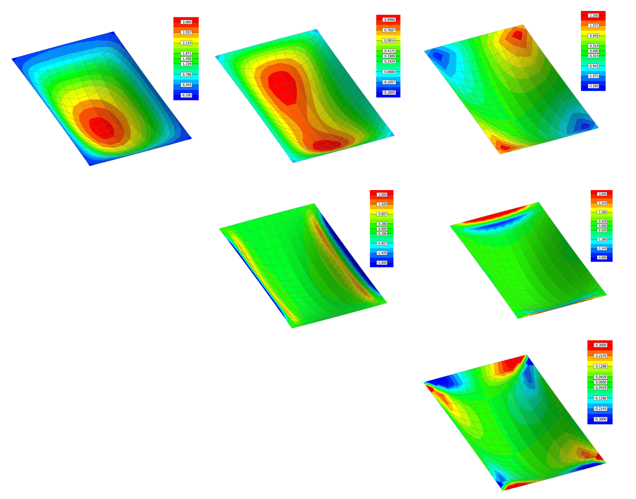
Image: coupling and many stiffness terms in matrices can lead to a complex system. Plate under vertical load. Because bending and normal forces are coupled, in-plane forces develop. Simple bending capacity verification becomes in-plane shear and shear connectors verification when in-plane shear resists vertical loads. The engineer must also account for coupling factors and fully understand the system and the plane’s shear stiffness. Forces top row: bending x and y, and shell twist Mxy. Middle row: Nx and Ny. Bottom row: in-plane shear Nxy.
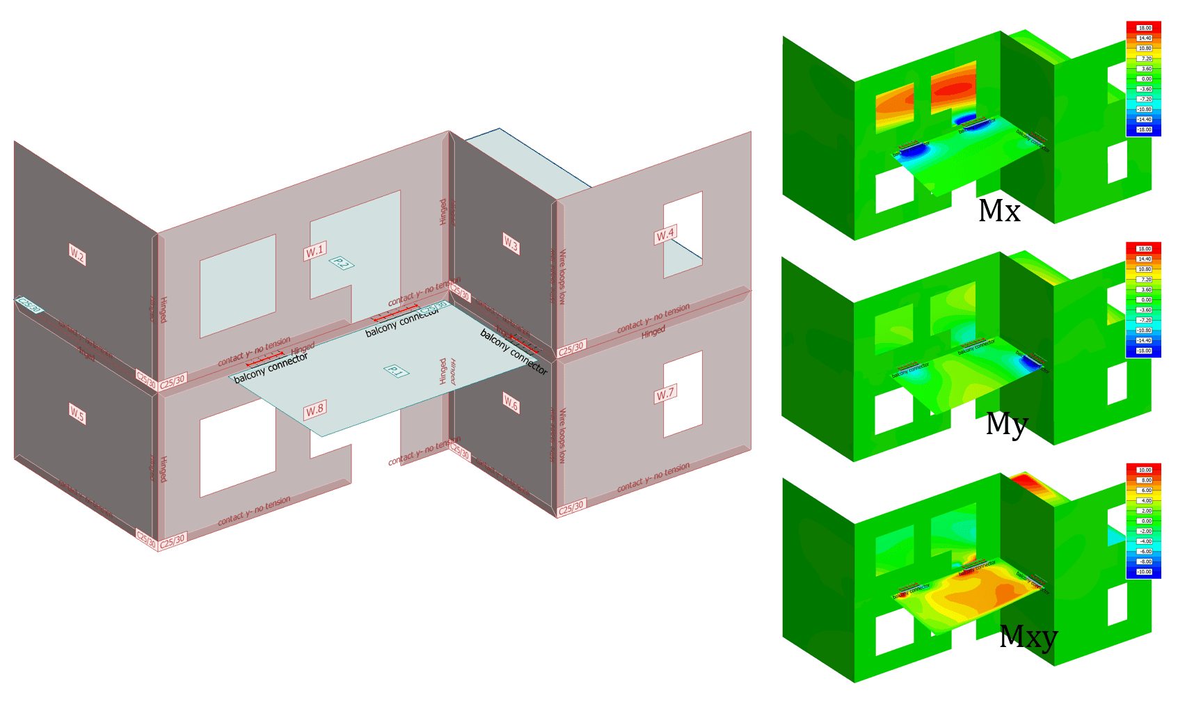
Image: Cantilever balcony plate calculation. Simplification of shell K matrix is not possible. Both bending terms Kx and Ky are needed and probably also coupling. Also, torsion stiffness KGxy is essential for the system’s response to get out correct Wood & Armer moments. And biaxial design of compressed concrete.
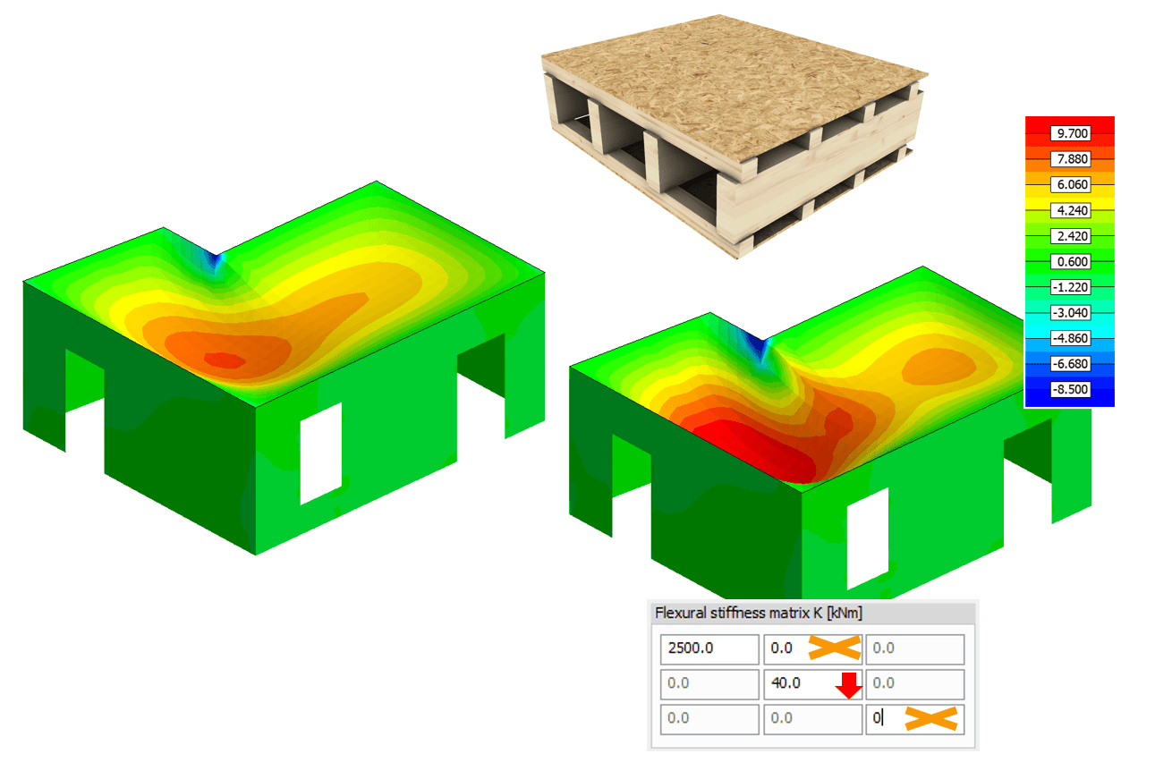
Image: One-way timber floor. A good case where simplification increases quality of calculation. Lots of uncertainty about shear stiffness of sheathing and its connectors and secondary stiffness of floor. When twist part and interaction part of the K matrix are eliminated, there is a lot less uncertainty about design moments of floor in the principal direction. Local yielding of deck connectors allows twist deformations.
Stiffness Adjusting, Cracking etc.
This blog covers linear shell analysis. Stiffness adjustment of shells can approximate the non-linear response of reinforced concrete. On the other hand, it can be used to model orthotropy. If bending stiffness is one quarter in one direction compared to the main direction, it is simply a 0,25 stiffness adjustment of the isotropic K matrix. Stiffness adjustments can also be used for local stiffness adjustments. Divide the shell model into a local area and adjust stiffness there to model a local opening, lower thickness, internal openings or whatever you might want to adjust. Stiffness adjusters can also be used to make a slab more uni-directional. It is all about understanding how stiffnesses change when a physical property changes in the structure. Usually, bending-related stiffnesses are very sensitive to the structure’s effective height (bending stiffness is proportional to the third power of the effective thickness). Some properties, like tension stiffness, are directly proportional to cross-sectional area. The same applies to thickness-direction shear stiffness. It’s proportional to thickness but also sensitive to geometry. Changes in the area of vertical parts better approximate shear stiffness than total cross-sectional area. Shear stiffness in the thickness direction also matters most in mid layers of plates.
When adjusting shell stiffness components, it should be noted that K and D matrices should be treated as a single entity – a mathematical model of the structure. One cannot simply tamper with one matrix factor and expect it to work as the user might think, especially when coupling is present, as is usually the case in linear continuous materials like concrete shells. Also, changing the Poisson ratio does not work as many think. Poisson’s ratio defines X-Y coupling and bending coupling. I have heard that many want to set the Poisson ratio to zero, as they have heard that cracked concrete shows zero Poisson ratio. This is true for a single point with in-plane forces in a single quad Shell FE. In bending, when cracking happens in one surface, the link between the two axes remains in the other surface. A better way to describe this is to use the FEM-Design materially non-linear model, where Poisson is set to zero only for those FEs where cracking strength is exceeded, and the model also sets the Poisson ratio on multiple layers in the thickness direction. So, one FE has multiple v values.
As such, whenever you adjust a continuous material shell model bending x term, you must also adjust the coupling terms. Otherwise, you break basic material properties (Poisson or compressibility). Look at the D and K matrix definitions above and the image below. Coupling terms are a function of Poisson’s ratio and the ratio of stiffnesses. Luckily, FEM-Design does this for you automatically if you use PLANE PLATE and PLANE WALL stiffness adjusters; coupling correction is done automatically.
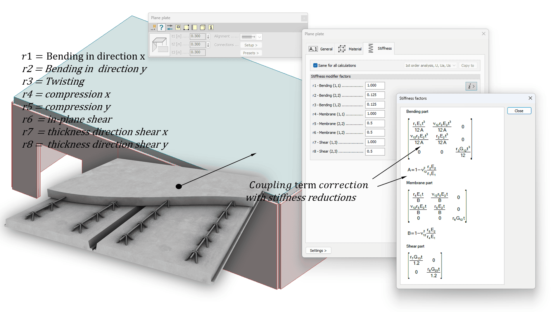
Image: Precast slab with surface casting approximation. Full bending stiffness in x-direction, surface slab stiffness in y-direction. Twist stiffness with surface slab. Reduced shear stiffness in y-direction. FEM-Design corrects coupling terms automatically. If the user wants to tamper with coupling terms, the shell can be converted to a fictitious shell: see next topic below.
For cracking-effect approximation in second-order analysis, EN 1992-1-1:2022 gives the following simplifications (image below). These can be added to all components of stiffnesses if exact loading is unknown. But these factors are just guidance. A wall under tensile load is not a wall – It is a tension tie, and stiffness loss caused by cracking is much higher than these code recommendations. For cracking of walls with twisting loads, roughly the same factors can be used as for a slab for bending – twisting is a bending-related phenomenon. For shear walls or floor diaphragms, it is closer to in-plane shear behaviour (wall recommendations). However, these kinds of guidelines are very inaccurate. Floor diaphragms seldom have constant shear throughout, and high shear and tension areas are very local – total in-plane shear stiffness is probably much closer to the uncracked state.

Image: Some guidelines for second order effects in EN 1992-1-1 (2022) annex O. The same kind of approximations can be used to correct a shell in ULS. For SLS consider tension stiffening models or non-linear calculation (FEM-design plastic or Cracked section analysis).
Automatic Shell Models
Many FE users live perfectly happy lives without fully understanding everything discussed in this blog. Usually, FE software defines these matrices D, K, B for you, and FEM-Design does exactly this. Just press the PLATE button in FEM-Design or TIMBER PLATE, select CROSS LAMINATE COMPOSITE material models, and everything is handled for you and factory default settings for coupling and matrices are set on the safe side. Below is an example of how orthotropy is also handled for you with coupling terms. The user draws a plate and selects GLULAMINATE timber material – it’s automatically an orthotropic shell with wood grains running in the x direction of the shell.
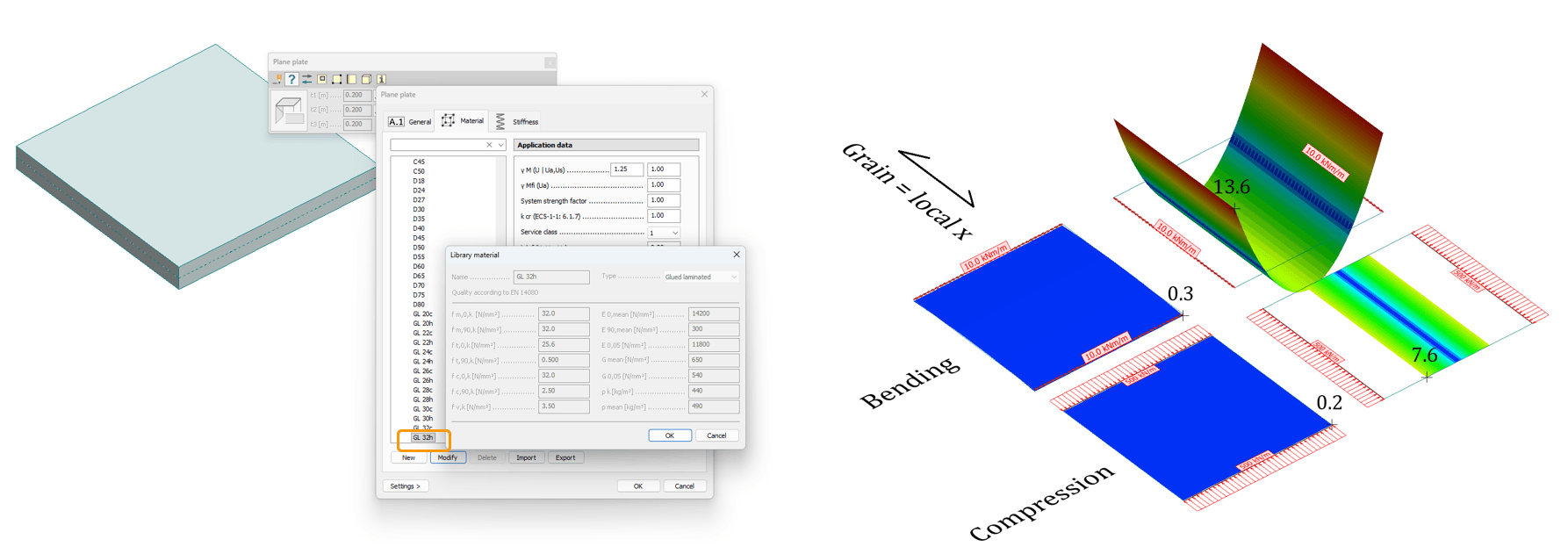
Image: Example of auto-generation of K and D matrices. Example of dramatic orthotropy of timber structures.
What if you are not happy with the model above? Do you believe that coupling terms should be different? y-stiffness should be 20% less? What if you want a concrete slab with coupling with bending loads but not coupling in in-plane forces? Maybe you want to match hand calculations of beams – and change to a simple Kirchhoff-Love shell model – increase thickness-direction shear stiffness to a high value. The good news is that you can convert everything to a FICTITIOUS SHELL. With a fictitious shell, D and K matrices are all yours. You can tamper with whatever you want. If a fictitious shell is hard to understand, first make a timber plate, RC plate, steel plate, Hollow core, or whatever, then convert it to a fictitious shell, and you will see the bare stiffness-matrix components of shell FEs. Modify as you please.
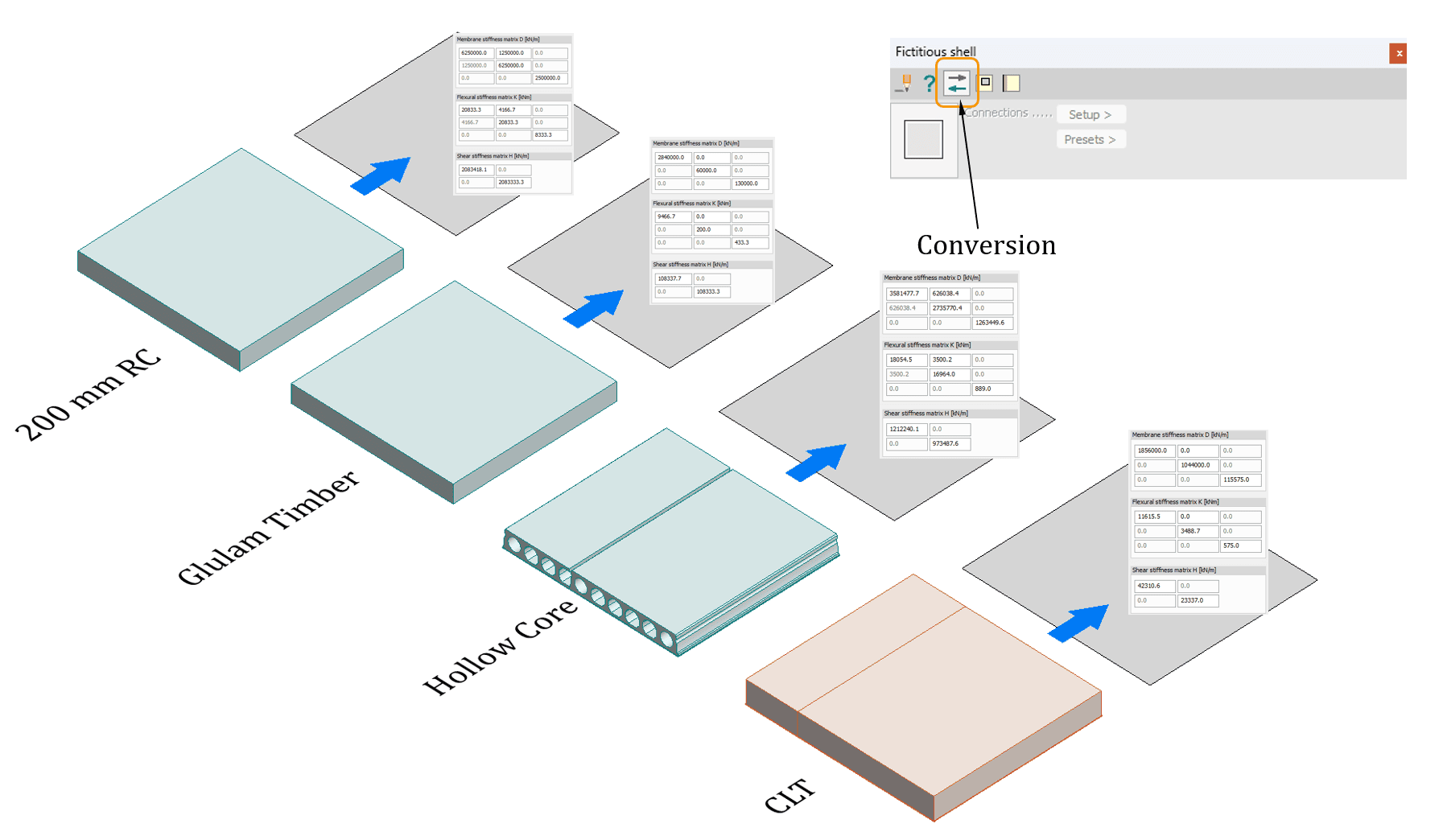
Image: Conversion of auto-generated shells to FICTITIOUS SHELLS as a starting point for a very custom shell FE. Please note that not all stiffness matrix properties are fully preserved. For example, Hollow core secondary stiffness presents since HC slab stiffness, not HC floor system’s stiffness.
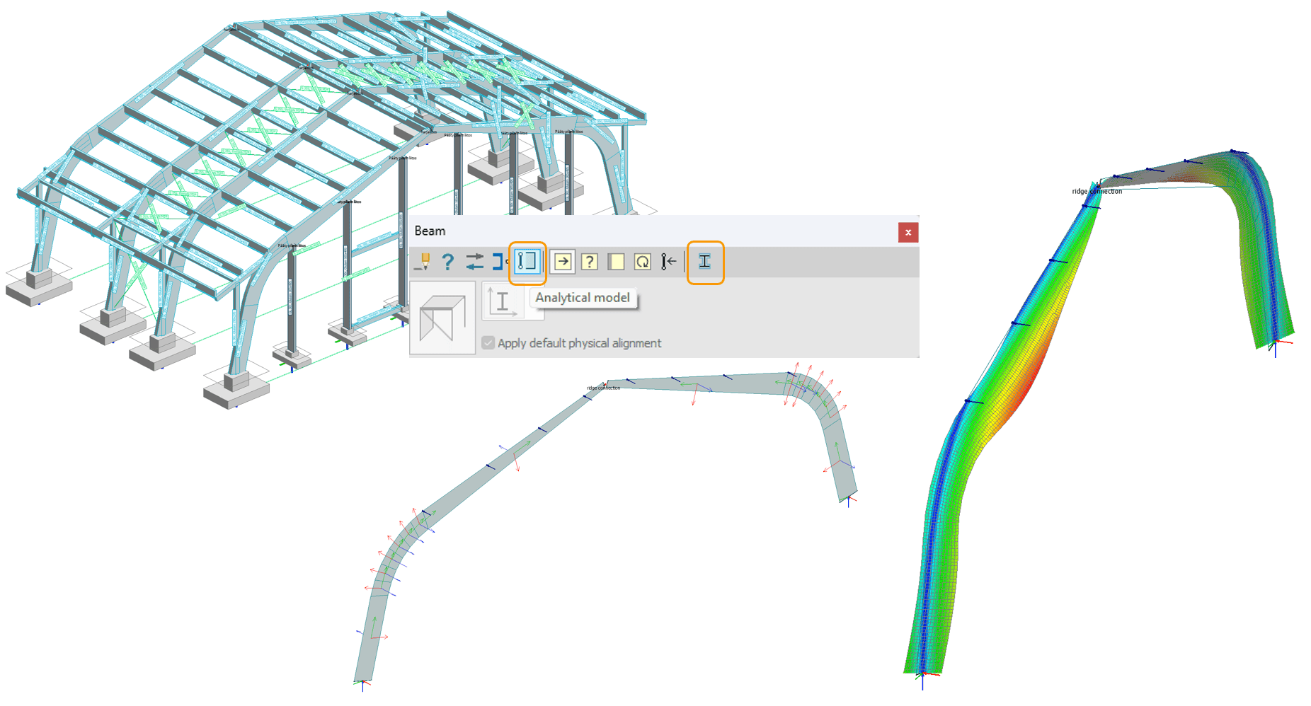
Image: Auto-conversion from beam model to orthotropic shell model. Wood grains follow beam axes. Lateral stability of Glulam with a detailed model.
Hope this shines some light on this complex topic. Often, we are ignorant of the beauty of the world behind the mathematical tools we use daily without a second thought. These are just building blocks – properties of those triangles and quads of the FE mesh. From here, the next step is to start building those engineering systems. Maybe more about that later if you are interested.
Author: Joni Hytönen